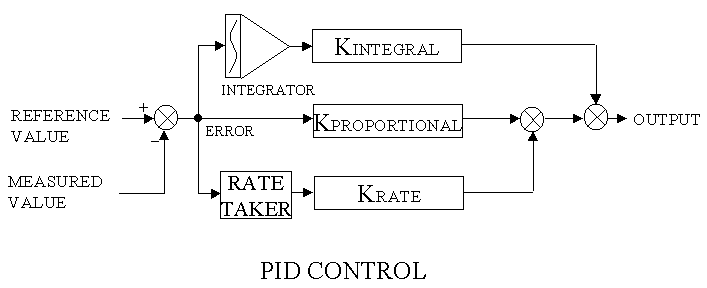
The following figure shows all three terms put together. It shows that by having just a single measured input signal, you can have proportional, derivative and integral components to your control. It becomes just a matter of selecting the right gains for each path. And we’ll go into that more later.

Unfortunately, there is a little bit more to it. The above drawing is a nice mathematical representation of how PID can be used. It is basically an ERROR correcting system, not necessarily a full range control system. It works best at providing an output to control a system which is already running at approximately the right value. It also works best for LINEAR systems. That is, systems whose output is proportional to the input. For example, if a robot's speed increases proportionately to the input voltage to the drive motor, say 10 inches per second per volt, the robot's speed control is linear. But, we know there are limits to the robot's speed. You can't increase the output beyond the battery voltage and friction or other loads may affect the speed of the robot. These are non-linearities which the above diagram does not cope with very well.
The next page will provide you a simulator where you can experiment with the basic PID equations in a linear environment. After that, we'll go into designing real robot drive and steering systems and show some of the tricks you can do to deal with non-linearities.
Software to implement PID would look like:
INTEGRAL = 0
LOOP:
ERROR = REFERENCE_VALUE - MEASURED_VALUE
RATE = (ERROR - ERRORLAST) / COMPUTATION INTERVAL
ERRORLAST = ERROR
INTEGRAL = INTEGRAL + ERROR * COMPUTATION INTERVAL
PROP = KPROPORTIONAL * ERROR
DERIV = KRATE * RATE
INTEG = KINTEGRAL * INTEGRAL
OUTPUT = PROP + DERIV + INTEG
ENDLOOP
Return to the Control law menu to select the next subject