Now it's time to start using this knowledge to build a control system.
There are several things you have to understand clearly to design your system properly:
What is the performance you want to achieve?
What range does the system have to operate over?
What are the characteristics of the hardware that you are
trying to control?
What sensor input is available to feedback the results of
your control?
What is the environment your robot has to operate in?
You don't necessarily have to know the exact numerical values of all the above, but at least the basic characteristics.
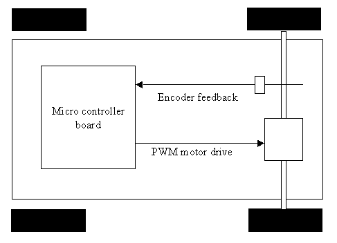
Let's try a new control, motor speed control (I assume we're all getting tired of steering for a while). To make it simple, let's assume a robot which has four wheels, doesn't turn, and has a single motor directly turning the rear wheels. There is a separate encoder measuring the wheels.

Motor characteristics:
Maximum
Speed: 240 RPM No
load (4 revolutions/second)
Stall
torque:
10 inch-pounds
Encoder characteristics:
128 pulses per revolution
Quadrature encoded
Microcontroller characteristics:
Uses interrupts (or separate hardware
counter) to count encoder pulses
Uses 2nd channel of quadrature encoder to increment count for
forward and decrement in reverse
Can count off the time between successive pulses and store
that time in a register.
Probably has an H-bridge between the processor and the motor.
Robot characteristics:
Wheel diameter: 3.2 inches for a
circumference of 10 inches
Wheel turns once for each motor and encoder revolution
Robot weighs 10 pounds
Initial assessment:
From the basic motor and wheel sizes, it appears the robot could have a maximum speed of 4 RPS * 10 inches (no load motor max speed times wheel circumference) = 40 inches per second. In reality, the robot will only reach this if it is going downhill as the friction of driving the robot will prevent the motor from reaching its no load speed on the level.
The stall torque of 10 inch pounds and the wheel radius of 1.6 inches says the robot will have an initial push of 10/1.6 = 6.25 pounds which should be plenty to get going under most reasonable condition and to climb some pretty good slopes (at least 30 degrees).
As an aside, one method I've used to estimate torque requirements is to place the robot in the environment of interest (e.g. a hard floor, a shag rug, up against a speed bump), and then use a string and scale to measure how much force is necessary to pull the robot forward. This method works well for getting the torque necessary to start as you just slowly increase the force until it moves. To get the torque requirement when moving at top speed is more difficult, but you can try to pull the robot along while reading the force.
One more thing to be aware of, is that available torque is inversely proportional to RPM You get stall torque at 0 rpm, and zero torque at no load maximum rpm. And torque decreases linearly as RPM increases. So, the robot won't be climbing a 30 degree slope at high speeds, but it should be able to crawl up. In general, your robot can go fast or it can be strong...but it can't do both at the same time. But, you can select a motor with enough excess power to go as fast as your want and as strong as you want at the same time.
So what does the control loop look like?
First, you have to make a decision as to what you are controlling to? That is, what are the units of your command signal. You can choose to command the speed of the motor, or you can command the position (distance traveled) of the motor. You COULD choose to control acceleration, or torque etc., but speed and distance are most common.
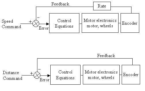
In each case, there is a command (coming from your navigation software), which is compared to a feedback signal from the wheel encoder. The feedback is either distance traveled, a count of the encoder pulses (converted to the same units as your distance command), or the wheel speed, determined from timing how often encoder pulses are received. The "Rate" block in the top diagram represents hardware or software that changes the encoder pulses into a speed (rate) signal.
The Control equations generate a PWM command signal which goes to the motor electronics (H Bridge) to drive the motor, wheels and encoder.
So, let's do the speed system first. We'll say that the Speed Command only commands forward velocity and can vary between 0 and 40 inches per second. The output, PWM duty cycle, can vary from -100% to 100%. First, we'll try a simple proportional control.

Just to go through it quickly; the Speed Command from the navigation software is on the left and is scaled in inches per second. As we stated above, the maximum speed of the robot would be 40 inch/sec or less; therefore this signal would normally vary from 0 to 40 ips. (or perhaps -40 ips to +40 ips if you want reverse also) The current actual speed comes from the rate block at the top and has been scaled to also be inches per second (ips) The two signals are subtracted to give an error signal (in ips) which is positive when the command is greater than the actual speed.
A proportional gain has been selected (somewhat arbitrarily) to be 5% of PWM duty cycle for each ips of error signal. Since the input can vary from vary from 0 to 40 ips, the signal can vary from 0 to 200% after being multiplied by Kprop. Since many PWM circuits may not work properly with an input of over 100%, it is best to add a limiter to ensure this can't happen.
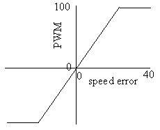 The limiter works as shown in the adjacent drawing. The PWM
command will increase with increasing error until the error signal reaches 20
ips and the PWM command equals 100%; after that, as the error continues to
increase, the PWM will remain constant at 100%. The
figure shows a limiter which limits for both +100%(forward) and -
100%(reverse).
Code for such a limiter is:
IF (PWMcommand > upperPWMlimit) THEN
PWMcommand = upperPWMlimit
IF (PWMcommand < lowerPWMlimit) THEN PWMcommand =
lowerPWMlimit
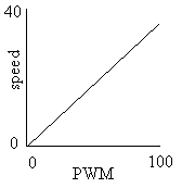
Now, what can we expect the performance of this system to be? First, lets look at one more plot. The adjacent drawing shows the expected steady-state speed as a function of PWM duty cycle. It shows a top speed of 37 ips at 100%.
Note that the max speed is equal to 0.37 times the PWM and, conversely, the PWM is 2.7 times the max speed. (we'll use this later)
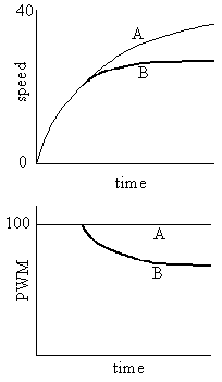 Normally,
applying a fixed PWM duty cycle to a drive motor will cause an increase in speed
which exponentially approaches the maximum speed for that duty cycle. In
the two adjacent drawings, the increase in speed for 100% duty cycle is
shown by curve A. It starts out accelerating rapidly (where friction is
least and the motor torque is greatest) and reduces acceleration over time as
friction builds up and the motor torque decreases. The speed eventually
becomes steady at a value of 37 inches per second where friction equals the
available torque.
But, the proportional system above doesn't quite work like that. If a 40 ips Speed Command signal is applied, the equations will generate a 100% duty cycle until the actual speed exceeds 20 ips, and hence, the error signal becomes less than 20 ips. Multiplying "less than 20 ips" by Kprop (5%/ips) no longer generates 100% duty cycle command, so the robot accelerates less rapidly.
Just to play a little math, we can predict what speed the robot will stabilize at:
From the speed vs PWM plot above: PWM = 2.7 * speed.
and from the control equation, PWM = 5.0% * speed error , which is the same as,
PWM = 5.0% * (Speed Command - speed) where Speed Command = 40
Hence, 2.7 * speed = 5 * (40 - speed) which when solved, gives speed = 26 ips.
Curve B shows how the acceleration and PWM reduce at speeds above 20 ips and stabilizes at 26 ips.
So, what this example demonstrated is that a pure proportional control law will not (and can not) reach the commanded speed since an error is necessary to maintain the PWM duty cycle command output. If the robot reached 40 ips (maybe with a push), the error would go to zero and zero PWM would be commanded, so the robot would decelerate. Note that this performance deficiency occurs because a drive motor system as described above requires a STEADY-STATE non-zero value of duty cycle to maintain any speed. And, in a proportional only system, an error signal is the only way to maintain that non-zero value. Hence, there is inherently an error.
Other control laws, such as steering, where any robot direction can be maintained with zero signal to the steering, may be able to work acceptably with just a proportional gain since no error signal may be necessary to hold a direction.
So, how are we going to get rid of this error and drive the robot to the commanded speed? Two methods are commonly used. Using the classical PID equations, it is POSSIBLE to generate a steady-state PWM command as the output of the integral term. Another method is to use a "Feed Forward" term. We'll do an example using the integral term first and then show how the feed forward term solves some of the problems we'll find.
The new control laws are shown in the following block diagram. The proportional part is the same as in the previous example; the integral part is as described earlier and with another relatively arbitrary gain of 0.5% /ips sec. To clarify, the integrator output will increase at a rate of 1 ips sec for each inch per second of speed error for each second that the error exists (actually, you could say that the integrator output is in inches, but I think it loses something in that translation). The output of the integrator is multiplied by the integral gain (Kint) of 0.5% duty cycle / ips sec. The gain value chosen is one tenth that of the proportional gain. This gain is necessarily low as the integrator tends to be quite destabilizing in this case.
The outputs of the proportional equation and the integral equation are summed together before being limited since the output should not exceed 100% regardless of where it came from.
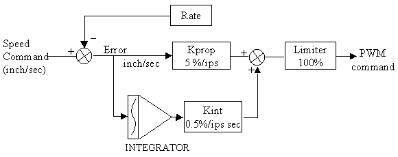
And how can this new configuration be expected to react to the same command to go directly from zero to 40 ips? Lines A and B are the same as in the previous plots for the Proportional gains. Line C represents the new configuration.
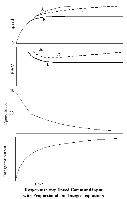
Comparing these plots to the previous ones, the first thing you should notice is that the speed finally does get to the maximum speed achievable with 100% duty cycle of 37 ips. Above 20 ips, the PWM again drops off since the Proportional command starts to decrease. But, since there is an error, the integral equation continues to increase until finally the total PWM command reaches 100% hence causing the robot to reach maximum speed.
While the robot finally reached its maximum speed, it took quite a while to do it. This is because the integrator gain must be fairly low to maintain stability. Certainly, since we know it could have reached that speed much faster by just setting the PWM to 100% and following curve A, the performance is not optimal.
Another characteristic which is less apparent on these drawings, but will be clear when you think about it, is that the integrator does not stop increasing its value at the end of these plots. There is still an error of 3 ips (40 commanded - 37 actual). Hence the integrator will keep running and generating more PWM command. Since the limiter keeps the PWM to 100%, the robot will remain at 37 ips, but the integrator will eventually have far more PWM command stored in it than the 100% required. This can become a big problem when you decide to decrease your Speed Command since the integrator will have to be driven down a long way before the PWM command will come off the 100% limit. This problem requires logic to be added to stop the integrator when it should not be running.
Another thing you may notice is that the reduction in PWM does not occur at exactly 20 ips, but is a little later. This is because the integrator has been running during the initial acceleration and when the proportional command becomes less than 100% (at 20 ips), the SUM of the proportional and integral gains still exceeds 100% for awhile.
While the second integrator characteristic above may be considered beneficial since it does cause the robot to accelerate faster, in general, an integrator should not be running when the output is limited since you really don't know whether an integral value will be needed until the system has stabilized. A simple solution is just to put the integrator in HOLD when the PWM limit is reached. However, since we do want the integrator to be able to run in the direction to move off the limit, a better logic is:
Don't run integrator
more positive if system is on +100% limit, and
Don't run integrator more negative if
system is on - 100% limit.
A sample pseudo code for the above would be:
LOOP:
RATE = (ENCODER - ENCODERLAST) / COMPUTATION INTERVAL
ENCODERLAST = ENCODER
ERROR = SPEED_COMMAND - RATE
IF ((ERROR > 0 AND PWM_COMMAND <=
upper PWMlimit)
OR (ERROR < 0 and PWM_COMMAND >= lowerPWMlimit))
THEN
INTEGRAL = INTEGRAL + ERROR *
COMPUTATION INTERVAL
PROP = KPROP * ERROR
INTEG = KINT * INTEGRAL
PWM_COMMAND =
PROP + INTEG
IF (PWM_COMMAND > upperPWMlimit) THEN PWM_COMMAND =
upperPWMlimit
IF (PWM_COMMAND < lowerPWMlimit) THEN PWM_COMMAND =
lowerPWMlimit
ENDLOOP
Note that logic has been added to keep the integrator from driving the PWM command farther into its maximums.
ANOTHER APPROACH
While it may be possible build a system with just proportional and integral terms that works well enough for your requirements, it is easy to build a system that has better performance. This can be done by adding a FEED FORWARD term.
A feed forward can also be explained by comparing to the way you drive a car. When you are driving down a straight road and come to a curve, you don't wait until the car starts moving away from the center of the lane before you move the steering wheel. You watch the cars approach to the corner and, at the right moment, you turn the steering wheel an estimate of the amount required. This gets the car moving in the right direction, and hopefully close to the center of the curve. Then you go to correction mode where you basically hold the wheel in the estimated position and make small corrections (proportional, derivative and integral) to maintain the center of your lane during the curve. (I also teach race driving, this is almost the same way I tell those people.)
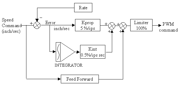
When a control system requires a steady-state value of output to maintain the desired performance, it is often possible to make an estimate of that value and add that to the equation. For the robot above, since we know maximum speed is 37 inches per second and that maximum speed occurs at 100% duty cycle, then we can calculate that the output will be about 100/37 = 2.7 % per inch per second of command. This estimate will often not be very accurate at low speeds since it takes a certain minimum PWM to get moving. You can make a better estimate by actually measuring how fast the robot goes for various applied PWM duty cycles. Just set the PWM to various fixed numbers and record what speeds they stabilize at.
You may get a plot that looks like:
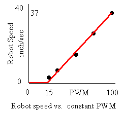 which
you can approximate with an equation like:
FeedForward = 15 + 2.3 * SpeedCommand.
So, the Feed Forward block above computes the above equation using Speed Command (not error) as an input and generates a PWM command which is a (hopefully close) approximation of the actual needed PWM.
So, how does this affect the robot's performance? The plots below show the new performance; but the thing to keep in mind is that now, the control equations will tend to generate higher PWM commands since you are ADDING to the previously calculated numbers. For our example of commanding 40 ips, the FeedForward alone will generate 107%. Hence, the motor will always be at full power and will get to its maximum speed of 37 ips as fast as it can. The proportional term will still be generating (40ips-37ips) * 5 = +15% and the integrator will still be at zero since the PWM was at 100% hence inhibiting the integrator. So, the total command is 107% + 15% = 122% which will keep the robot at max speed.
Considering the above, the previous example of a command of 40 ips is becoming a poor example since the equations aren't really doing any controlling anymore, they're just driving the motor at full speed (which is correct for this case).
So, let's try a better example to show the equations effect. The new commanded speed is 20 ips.
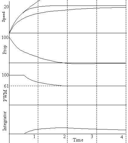
Just to get calibrated, the top line in the top plot of speed shows how quickly the target speed would have been reached if the motor had been run at 100% PWM. So, you can't do any better than that. The lower line in the top plot shows how the speed would have increased if the final value of 61% (15% + 2.3 * 20ips) had just been applied all the time.
The middle line shows how the speed would respond if the control laws above were used. A 61% feed forward was used and the second plot shows the output of the proportional term. Adding the two together and limiting at 100% gives the PWM plot. PWM goes to 100% until the speed is close to the target, then decreases to the feed forward term as the target speed is captured.
One minor characteristic worth noting is that the integrator did have a small impact on this performance. The integrator was inhibited (in HOLD) while the PWM was limited at 100%, but as PWM came off the limit, the integrator began to increase in value due to the error signal. Since the integrator gain is so low, it didn't change the PWM much, but you can see that the speed went slightly over the target value of 20. This caused a slightly negative proportional term which was necessary to cancel out the integrator term. Over time, the slight negative (overspeed) error would cause the integrator to run down toward zero and the robot to get right on speed. This is another indication that you have to keep your eye on what integrators are doing in your system. The performance, in this case, would have been more accurate without the integrator. If there are significant errors due to the integrator, you may be able to correct or reduce them with different logic controlling the HOLD function of the integrator; like not turning the integrator on until later.
However, an integrator can be very useful; especially in this kind of motor control system. The example above converged so quickly on the target speed because I assumed that the FeedForward value was very accurate. If the FeedForward was determined for a robot rolling on a hard level floor with a fully charged batter, the performance could be expected to be accurate as long as those conditions exist. But, running on a rough floor (shag rug?) would require more PWM, a reduced battery voltage would require more PWM and a sloped floor could require more or less PWM depending on whether it was uphill or downhill.
Lets do the example again assuming any or all of the assumed conditions were different and that a PWM of 75% would be required to go 20 ips.
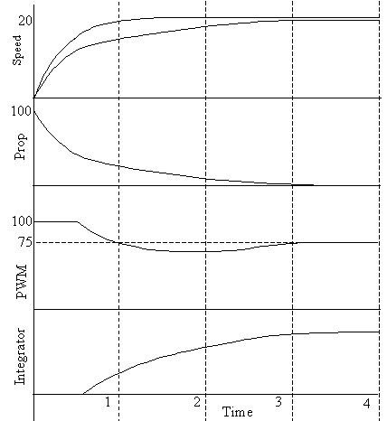
So, what changed. The first plot shows the performance from the last test (where the FF term was accurate) as the top curve. The lower curve shows the performance when the FF term is too low. It is clear that it didn't accelerate as rapidly, even when at 100% duty cycle, and didn't reach the target speed as rapidly.
You can see that the speed error is starting to level off at about the 1 second point. That speed error goes into the integrator which keeps running in the positive direction. Eventually that integrator term, added to the proportional and feed forward terms, creates enough PWM command (75%) that the motor reaches the target speed. At that time, the speed error reaches zero and the integrator stops increasing and holds the value necessary to maintain 20 ips.
In a similar manner, if the robot had been going downhill such that the PWM to reach 20 ips was only 50%, the robot would have accelerated more quickly and overshot the target speed, maybe up to 21 or 22 ips. This would have caused the integrator to increase in a negative direction and subtract from the total PWM command until the PWM got down to 50% and the robot reached 20 ips.
For most drive motor controls like this, a proportional gain, integral gain and a feedforward gain will probably give you good performance.
Some enhancements:
This system responds fairly well to commands that step (jump) from 0 to 40 ips or 20 ips, but it does have large errors while acquiring the new speed; and only reaches the new speed at maximum accelerations (100% PWM) which might not be what you want. Maybe we can compute a more reasonable reference for the equations to follow and get better control.
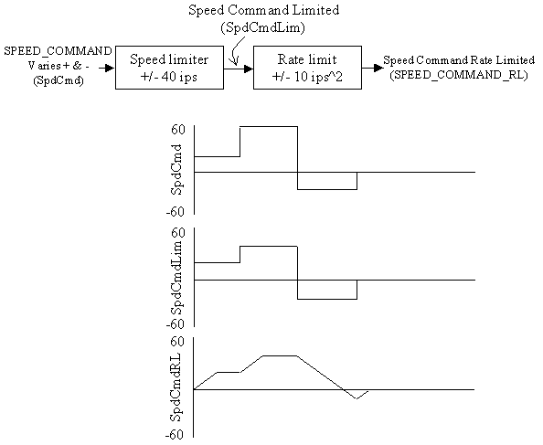
The first change, which has been assumed until now, is a speed command limiter at the beginning which ensures that the speed reference never exceeds the design parameters of the control equations. In this case, you might want to limit the speed to +/- 40 ips.
This can be implemented as:
IF (SPEED_COMMAND
> 40) THEN SPEED_COMMAND = 40
IF (SPEED_COMMAND < -40) THEN
SPEED_COMMAND = -40
Similarly, to reduce your robots speed changes from maximum PWM sprints to something smoother, you can add a rate limiter. Perhaps to limit your robot's acceleration to +/- 10 inches per second squared.
This can be implemented as:
RATE_LIMIT = 10 * computation interval
SPEED_CMD_ERR =
SPEED_COMMAND - SPEED_COMMAND_RL
IF (SPEED_CMD_ERR > +RATE_LIMIT
) THEN SPEED_CMD_ERR = +RATE_LIMIT
IF (SPEED_CMD_ERR < -
RATE_LIMIT ) THEN SPEED_CMD_ERR = - RATE_LIMIT
SPEED_COMMAND_RL =
SPEED_COMMAND_RL + SPEED_CMD_ERR
These equations will cause SPEED_COMMAND_RL (the rate limited speed command) to increase (or decrease) to a new speed reference at a maximum rate of 10 inches per second squared. Note that the RATE_LIMIT value is multiplied by your computation time interval so as to add the full value over one second.
This will generally allow your robot to follow the rate limited signal much more tightly since the error caused by changing the reference will be small at any given time.
A block diagram with a speed limiter and a rate limiter follows with plots showing response to a step input:
Performance accuracy can be improved even more by adding another feedforward term. We knew that the motor would require a certain amount of PWM to roll along at any selected speed. The FeedForward term used previously added this value. The robot ALSO requires some additional PWM to accelerate. For example, the PWM required to be steady at 20 ips in the example above (61%), is less that is required for the robot to be at 20 ips and be accelerating at 10 ips^2. We can come up with an estimate of the power required for acceleration and add that as another feedforward. Conveniently, the rate limiting equations above have a variable which is the acceleration commanded at any time: SPEED_CMD_ERR.
So you just have to add another feedforward term as in the block diagram below.
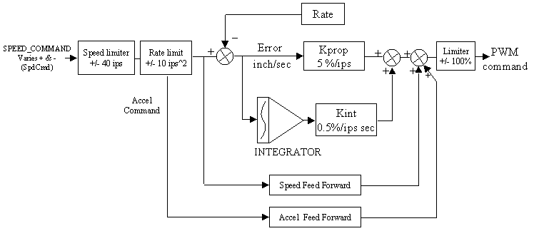
You can make an estimate of the accel FeedForward gain by running your robot and applying step speed command inputs (which are converted to ramp inputs by the rate limiter). Record the rate limited commanded speed and the current actual speed as the robot accelerates. If the actual speed is generally less than the commands (during the acceleration phase), the accel feed forward gain is too low. If the actual speed is generally above the ramp command, the accel feed forward is too high. Just adjust the accel FF gain value until the robot's actual speed tracks the command best.
The above block diagram and associated equations (following) should give you good control on your robot's speed.
We've described methods to determine the two FF gains, but not the Kprop and Kint gains. Those two gains should be as high as possible without affecting the stability of the system. I hope that by using the PID simulator earlier, you got a feel for the effects of changing the three PID gains.
By the way, since this control (a drive motor) produces an output (speed) which is basically proportional to the control (rather than the integral of the control as occurs in car type steering systems), no derivative gains was necessary.
A full set of pseudocode for the above block diagram follows
LOOP:
IF (SPEED_COMMAND
> 40) THEN SPEED_COMMAND = 40
IF (SPEED_COMMAND < -40) THEN
SPEED_COMMAND = -40
RATE_LIMIT = 10 *
computation interval
SPEED_CMD_ERR =
SPEED_COMMAND - SPEED_COMMAND_RL
IF (SPEED_CMD_ERR > +RATE_LIMIT
) THEN SPEED_CMD_ERR = +RATE_LIMIT
IF (SPEED_CMD_ERR < -
RATE_LIMIT ) THEN SPEED_CMD_ERR = - RATE_LIMIT
SPEED_COMMAND_RL =
SPEED_COMMAND_RL + SPEED_CMD_ERR
RATE = (ENCODER - ENCODERLAST) / COMPUTATION INTERVAL
ENCODERLAST = ENCODER
ERROR = SPEED_COMMAND_RL - RATE
IF ((ERROR > 0 AND PWM_COMMAND <= upper PWMlimit)
OR (ERROR < 0
and PWM_COMMAND >= lowerPWMlimit)) THEN
INTEGRAL = INTEGRAL + ERROR *
COMPUTATION INTERVAL
PROP = KPROP * ERROR
INTEG = KINT * INTEGRAL
SpeedFF = SPEED_COMMAND_RL * KFFspeed
AccelFF = SPEED_CMD_ERR * KFFaccel
PWM_COMMAND =
PROP + INTEG +
SpeedFF + AccelFF
IF (PWM_COMMAND > upperPWMlimit) THEN PWM_COMMAND =
upperPWMlimit
IF (PWM_COMMAND < lowerPWMlimit) THEN PWM_COMMAND =
lowerPWMlimit
ENDLOOP