This will be REAL basics. Only a couple definitions so you can follow the later pages. Like, what a Derivative and and Integral actually are; and how to do differentiation and integration in software. There will be NO math except basic algebra and geometry.
Derivative:
This is simply the rate of change of some
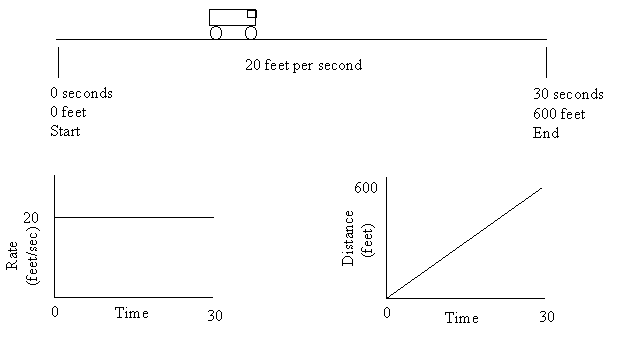
signal. Your car may travel forward at 20 feet per second for 30
seconds. It will travel 600 feet. During that 30 seconds, the distance
the car has moved can be measured and will vary from 0 feet at the beginning to
600 feet at the end. The derivative of the distance measurement is the
rate at which it changes; which is a constant 20 feet per second during the
entire 30 seconds

It is possible that your car's speed could vary during the 30 seconds Maybe you drive up and down a hill with the gas pedal held constant, or maybe you push or release the gas pedal to change the speed.
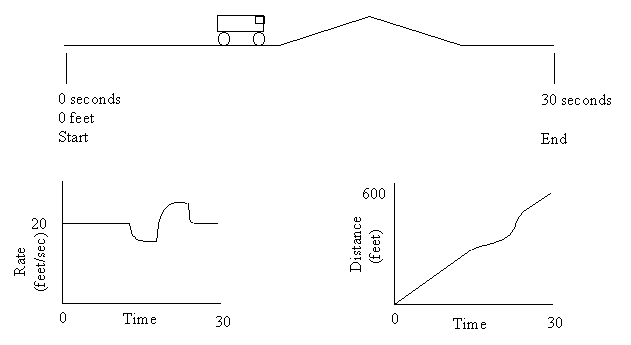
You can see that the car proceeds at 20 feet per second (fps) until it reaches the hill. Then it slows down to about 15 fps. As it tops the hill and starts downhill, the speed (rate of distance) increases to about 25 fps. Then when it reaches the level road again it returns to 20 fps. This change in speed can also be seen on the plot of distance versus time. The line (distance) increases at a constant rate (20 fps) until the hill is reached. Then the rate of increase in distance reduces until the downhill portion when it speeds up. Then it goes back to the original rate of increase ending up at approximately 600 feet again. (if you do the math, you'd find that it doesn't quite make it to 600, since you lose more time going uphill then you make up going downhill)
The rate plot is the derivative of the distance plot. The rate plot shows the speed or rate at which the car is covering distance.
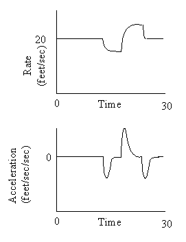
There is also a derivative of the rate plot. Since the second example with a hill results in a rate plot with different values on it, then the rate plot also changes as a function of time. The change in rate is acceleration. So, speed is the derivative of distance and acceleration is the derivative of speed. Actually, you can keep taking derivatives of derivatives forever, but we seldom have to worry about any derivatives beyond acceleration.
The plots on the right show that while rate is constant at 20 fps, the acceleration is zero. When the hill is encountered, there is a negative acceleration which is the rate signal decreasing to 15 fps. The acceleration returns to zero as the speed stabilizes at 15 fps. Similarly as the car starts downhill, there is a positive acceleration until the car stabilizes at 25 fps, then there is another negative acceleration as the car returns to level ground at 20 fps.
Integral:
The integral is just the opposite concept of the derivative. If you start with the acceleration, speed (or rate) is the integral of acceleration; and distance is the integral of speed.
For all these examples, we will be talking about signals that occur over time. So, if you have a measured signal that tells you (or your robot) how its speed has varied over an interval of time, you can calculate what distance the robot has traveled over that same period of time by multiplying the speed times the TIME that the robot spends at that speed.
Note: Two methods you can use to measure speed are a tachometer attached to the motor or drive train, or measuring the back-EMF of the motor (which is the same as using your motor as a tachometer). Of course, if you have wheel encoders, you could calculate speed from them and integrate that value to get distance; however, this is unnecessary since the encoder gives distance directly.
Since rate is often changing over time, you will usually calculate the distance traveled frequently, computing the distance traveled since the last computation and adding all the incremental distances together for a total. If this is done at a high speed, e.g. 20 times per second),. the resulting distance can be quite accurate.
There are two primary sources of error in computing distance from speed. First is the accuracy of the speed signal. If speed is off by 10%, distance will be off by 10 percent also. This error source can be minimized by doing a calibration of your speed signal to make it as accurate as possible. Second is the accuracy of the piecemeal integration. Multiplying current speed by the time since the last sample assumes the speed was constant over that time. If the speed increased or decreased, the answer will not be quite right. This source of error can be minimized by performing the calculation at such a high rate that the speed change between calculations is insignificant; or by using a value for speed that is the average of the current and previous values.
 For example, you have a robot and have some means of measuring its
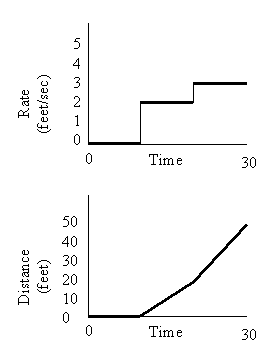
speed. You find that it moved at 0 fps for 10 seconds, then 2 fps
for 10 seconds, then 3 fps for 10 seconds. How far has the robot moved?
In the first 10 seconds, it doesn't move at all. In the second 10 seconds it moves 20 feet (2 fps * 10 sec) and in the final 10 seconds it moves 30 feet. Add it up and it is 50 feet. As plots it would look like:
SOFTWARE:
INTEGRATOR-
OK, assuming we have the concept down, how would you implement a calculation of the integral in software? The object is to integrate the rate signal to get the distance measurement.
As the robot runs, you are making the speed measurements each time your software executes. Lets assume your software executes at 20 times per second. Using pseudocode:
DISTANCE =
0
//Initialize DISTANCE integrator to zero
DO while time<30
seconds
//just for the length of the test
SPEED =
???
//however you measure the rate signal
DISTANCE = DISTANCE +
SPEED/20
//the actual integration
LOOP
This loop will execute 600 times, 30 seconds at 20 times per second. A new value of speed is determined for each execution. The distance measurement is then updated by taking the previous value of distance and adding how far the robot would move in 1/20 of a second at the measured rate.
The special characteristics of an integrator are: that it must be initialized since the computed value is always based on the previous value; and the amount added for each cycle of the integration must be multiplied by the time interval between executions (0.05 seconds or 1/20 of a second in this case).
This is all there is to an integrator. If you integrate an acceleration signal, you will get speed; if you integrate speed, you will get distance.
SPEED =
0
//Must also initialize Speed now
DISTANCE =
0
//Initialize DISTANCE integrator to zero
DO while time<30
seconds
//just for the length of the test
ACCELERATION =
???
//however you measure the accel signal
SPEED = SPEED +
ACCELERATION/20
//integrate to get
speed
DISTANCE = DISTANCE +
SPEED/20
//integrate to get distance
LOOP
Lest you get too carried away with this, integrating acceleration twice to get distance may work fairly well in the bowels of a high precision digital computer; but, trying it in the real world can lead to large errors. This is because your measured signal is probably not perfect. If you had an accelerometer on your robot measuring how fast it was accelerating forward or backwards, and that accelerometer was off by just .001 g's (.0332 feet/second^2), the integration of speed would be off by 1 fps and the distance integrator would be off by 14 feet. Hence, integrating navigation measurements to get position is not often done over prolonged periods of time. But it can be useful at times. For example, if you are measuring the distance traveled with a look-behind sonar, and the sonar quits providing data for a second or two, you may be able to keep your distance updated pretty accurately by integrating speed into the last valid sonar measurement.
By the way, a single integration of speed to get distance can be much more accurate since the error only builds up linearly with time rather than exponentially (squared) with the double integration.
While the example above of integration showed the concept, most actual uses of an integrator will be for short term navigation backup or for doing corrections in the control equations (the "I" part of PID). And the control equations are what will be discussed here.
Derivative-
Using software to get a derivative is also easy, and also has its own set of problems.
The most basic way to calculate the derivative of a signal is to subtract the previous execution cycle's value of the signal from the new value. For example, if your software is executing 20 times per second and you have just measured your distance (perhaps from an encoder) to be 98.6 inches; and the value on the last cycle was 97.8 inches; then you can calculate the speed (the derivative of distance) as (98.6 -97.8) * 20 = 16 inches per second.
You can do this over a 30 second interval by:
DO while time<30
seconds
//just for the length of the test
DISTANCE =
???
//however you measure the distance
SPEED = (DISTANCE - DISTANCE_LAST) * 20 //perform
differentiation
DISTANCE_LAST =
DISTANCE
//save the distance to use as last distance next loop
LOOP
Note that you didn't have to initialize SPEED as you had to initialize DISTANCE in the integral. This is because SPEED is recomputed each cycle and the previous value doesn't carry over. However, the first value of speed calculated will be wrong unless DISTANCE_LAST has been initialized to the correct value. And the sample code above doesn't even set DISTANCE_LAST until after SPEED has been calculated. If DISTANCE starts at zero, this probably won't be a problem. But, if you turn on the speed calculation when distance is perhaps 10 feet, and DISTANCE_LAST is zero because it hasn't been used yet, your first calculation of speed would be (10-0)*20 = 200 feet/second; which might cause a large command from your control equations. This problem can be overcome in several ways including: set speed to zero on the first time the speed calculation is done (if zero is an acceptable value for your equations); or set DISTANCE_LAST = DISTANCE for all processing loops, not just ones where SPEED is calculated (so it is already set when the first time the derivative loop is called); or set SPEED to a reasonable estimate of speed on the first calculation.
And the differentiation takes a TIMES 20 (rather than a DIVIDE BY 20 as in integration) because the difference in distance is what happened over just 1/20 of a second; and you want to compute how much distance would have passed over a whole second.
Now for the problems: the differentiation often has low resolution and is very susceptible to noise.
In the example above, the encoder distance only changed 0.8 inches over .05 seconds. If it has 0.1 inch resolution, then the derivative output only has 12.5% resolution (0.1/0.8). This isn't very impressive. And if you increased your execution rate to 100 per second, then the number of encoder pulses per cycle would be just 1 or 2 (0.1 or 0.2) inches. This means your derivative speed calculation would be jumping back and forth from 10 inches per second to 20 inches per second.
This isn't necessarily disastrous. First, the derived value often goes into a calculation which results in a PWM signal which inherently is turning on and off at a high rate and the motor dynamics filter that PWM signal into something which appears smooth. Hence, a noisy derivative may just cause the PWM signal to change its duration a bit noisily; but the motor will filter the noise out giving the right average value. Another alternative, if you find your calculations bouncing around to be distasteful, is to filter or average the derived signal.
Averaging is easy to do, just save the last few values, add them together and divide by the number of values added. A low pass filter (which I hope to go into later) will also smooth the signal output. The disadvantage to averaging or filtering is that the data you are using is not the most recent. If you average 5 values, the data resulting is about what the data was 2 cycles ago, not what it is now. This time delay can cause oscillatory problems in high speed high gain calculations. Hopefully, we can avoid such problems, but the time delay factor is something to keep in mind. The best plan is to use the shortest period of averaging or filtering that will give acceptable results.
Return to the Control law menu to select the next subject