The examples of pure proportional control showed that a robot with car-type steering was not capable of returning to the reference line and staying there. It oscillated from side to side. This problem can be corrected by adding the derivative term to the equations.
If you are driving a car and find that you have drifted four feet off to the right of your lane, the first thing you do is turn the steering wheel to the left to head back toward the lane. And you probably just turn the wheel left for a moment until the car turns a bit and is heading back to the lane, then you probably return the wheel to center. As the car moves left, you note that at its current RATE of moving left, you will reach the center of the lane soon and drive over to the other side. So, to slow down the rate, you turn the steering wheel a little to the right to reduce the rate of motion to the left. As the car reaches the center of the lane, you reduce the amount of right steering wheel until the car is right in the center of the lane with no sideways motion.
The Proportional and Derivative terms do just what you did in the example above, but it smoothes it into one continuous maneuver. The proportional term says to turn left to get to the center of the lane, the derivative term says to turn right so as not to be moving across the lane. The two terms will balance out so that a large distance from the lane is balance by a large rate approaching the lane center, and a small displacement from the center is balanced by a small rate.
The block diagram of a PD control law follows, set up to follow a wall as in previous examples:

steering command = Ksteering * (reference distance – sonar distance) + Krate * rate
What this equation provides is guidance to make an asymptotic approach to the reference. Both the distance error signal and the rate error signal are trying to drive the steering to make themselves equal zero. What will happen is that the steering will turn such that a proportion is held between distance and rate. The proportional gain is trying to make the robot turn toward the reference line and the derivative gain is trying to make the robot turn to be parallel. So if the robot is approaching the line from the left, proportional is trying to make a right turn, and derivative is trying to make a left turn. At some point the two will balance, and if this balance point is followed, the robot ends up on the line. For example in the block diagram above, where the steering gain and the rate gain are both the same magnitude, the steering will balance out when the rate is equal to the distance. If the robot is 12 inches to the right of the reference, and is moving to the left at 12 inches/second, the steering will be zero. As the robot continues to the left until it is 6 inches away, the rate signal, now being proportionately larger than the distance will cause the steering to turn to the right until the rate is just 6 inches per second when the steering command would again be zero. Similarly, as the robot approaches to 2 inches on the right of the reference, the rate will be reduced to two inches per second; and as the distance error reaches zero, the rate will also be zero. Hence the robot will be traveling parallel to the wall at the right distance. As the control equations are computed many times a second, the resulting path will be smooth rather than the occasional turn implied above.
This new equation will work for both the differentially steered robot and a car-type steering robot. However, they won't follow exactly the same path to get there since the differential steering robot pivots immediately to point in a new steering direction, and the car-type steering robot must move forward some distance to turn toward the reference line.

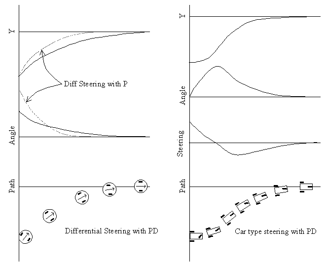
The two plots above compare the performance of a differential steering robot with a car type steering robot. Note that both turn toward the desired path and turn smoothly onto it. The difference is that the differential steering immediately turns the robot toward the target path and then slowly turns back to the right until it is centered on the path; while the car type steering must first turn the robot left toward the path and then turn right to straighten it out onto the path.
For those of you still picking up on Integrals and Derivatives, you may notice that, in the car type plots, the robot Angle is the integral of the Steering plot, and the distance from the line, Y, is the integral of the robot Angle. That is, the Angle is the rate of change of the distance, and the Steering is the rate of change of the Angle.
The dashed lines in the differential steering plots show what the path of the robot was before when only the P term was used. The effect of the Derivative term was to reduce the rate at which the robot approached the reference path. The initial Angle was reduced when the D term was added since the command used to be just the proportional term and with PD, it is now the proportional minus the derivative.
In the case of the car type steering, a P only control resulted in continuous oscillation. The PD configuration provides a stable capture of the reference.
Return to the Control law menu to select the next subject